Fault Injection: Proving Diagnostic Coverage Instead of Claiming It

Every FMEDA has rows like this one: the 1.2 V core supply of the main microcontroller, a failure rate from the reliability handbook, safety mechanism "window voltage supervisor", diagnostic coverage 99 %. The number usually comes from ISO 26262-5:2018, Annex D, which rates monitoring of a supply output as able to reach high coverage, and high corresponds to about 99 %.

Annex D is clear that its values are a starting point. They describe what a type of mechanism can typically achieve, not what this supervisor, with these thresholds and this filter, achieves on this board. The claimed number needs a rationale, and the standard names two kinds: analytical arguments and fault injection. A table value with neither behind it is a claim, not evidence.

Where fault injection sits

ISO 26262-1:2018, Clause 3 defines fault injection simply: put a fault into an element and watch the reaction at chosen observation points. ISO 26262-5:2018, Clause 10 lists it among the hardware integration tests, highly recommended at ASIL C and D. ISO 26262-11:2018, Clause 4 describes how it supports the evaluation of diagnostic coverage and of the time a mechanism needs to detect a fault and react. An analytical argument can carry a coverage claim too, if it works through this filter, these thresholds and every failure mode. What injection adds is that it tests the mechanism as built, including the parts nobody thought about when the coverage figure was written down.

A supervisor on the bench

The supervisor in this example watches the rail through a window of ±4 %. So that it does not reset the microcontroller on every load step, it only reacts once the rail has stayed outside the window for 40 µs. The team builds a campaign on the bench: undervoltage and overvoltage steps from a programmable supply, slow drifts, and spikes from a pulse generator. 300 injections, 300 detections. The test report says 100 %, which looks comfortable next to a claim of 99 %.

Annex D names the failure modes to consider for a power supply: under and over voltage, drift, oscillation and spikes. Oscillation was missing from the campaign, because the bench supply could not produce it. A second campaign adds it, coupling a 40 kHz ripple of ±7 % into the rail through an injection transformer. The supervisor never responds.

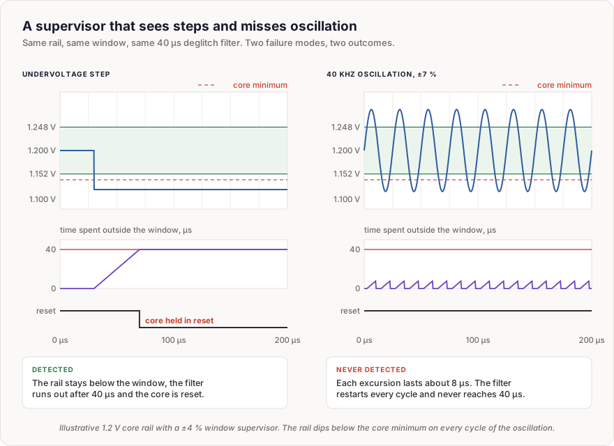
The reason is the filter. Each excursion outside the window lasts about 8 µs, the filter restarts every time the rail comes back inside, and it never reaches 40 µs. Meanwhile the rail drops below the core's minimum operating voltage on every cycle. The mechanism works exactly as designed and is blind to one of the four failure modes it was credited with. The second campaign also varies the spike width and shows that spikes shorter than 40 µs pass unseen. The first campaign could not see that, because every spike it injected happened to be longer.

Count failure rate, not injections

The tempting next step is to merge the results: so many detected out of so many injected, and call the ratio the coverage. That ratio depends on how many faults of each kind the team chose to inject, which is a test planning decision. A campaign that injects a hundred faults of a mode carrying 2 % of the failure rate and two faults of a mode carrying 40 % can report almost any number. Diagnostic coverage is something else. Part 1 defines it as a share of failure rate, and Annex D of Part 5 shows how to compute it for an element with several failure modes: each mode's coverage is weighted by that mode's share of the element's failure rate. The distribution belongs to the hardware, not to the test plan.

With an illustrative distribution of 55 % under and over voltage, 20 % drift, 15 % oscillation and 10 % spikes, the supervisor covers 55 + 20 + 0 + 5, about 80 % of the rail's failure rate. The 5 for spikes holds only because the second campaign spread its spike widths the way real spikes on this rail are expected to occur, and half of them were shorter than 40 µs. Inside a mode, the injections have to follow the failure rate as much as between modes, or the spike column repeats the counting error on a smaller scale.

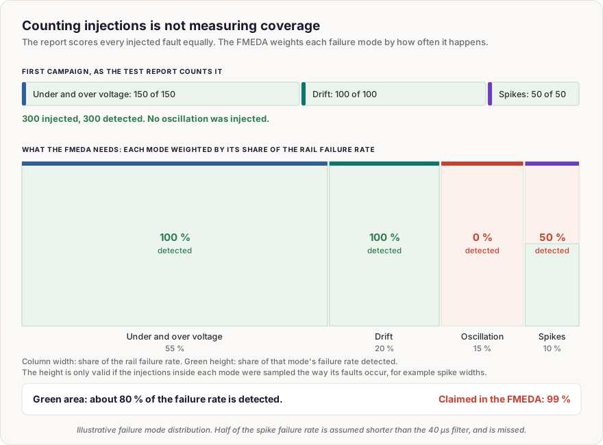
Eighty percent instead of 99 % means the undetected part of this element's failure rate is twenty times larger than the FMEDA assumed. That residual feeds the single-point fault metric and the probabilistic metric for random hardware failures, which the hardware metrics post explains. The team now has two honest options: change the mechanism, for example a shorter filter or a separate ripple detector, or lower the claim and check whether the metrics still close. Either way, the decision now rests on a number for this implementation instead of a handbook one.

The Fault Injection Testing concept page covers the fault models, the hardware, software and simulation techniques, how to plan a campaign and classify its outcomes, how many injections a coverage claim needs, a complete worked example from fault list to safety case entry, and the pitfalls that get campaigns rejected by assessors.